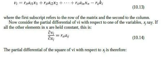
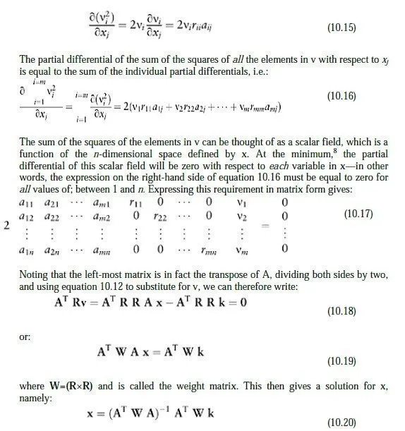
and now the goal is to find the values for x which give the smallest result when the scalar elements of v are squared and added together. It is clear at this stage that equation 10.12 can be used for problems involving more than three observations or two variables, as in our simple example. For bigger problems, v, R, A and k have a row for each measurement, with the elements in A and k being calculated from the initial guessed geometry, as shown in the example. The remainder of this explanation will therefore assume that there are m measurements and n variables, with m being larger than n. Consider now how the ith element in v is obtained from equation 10.12. We can write:

Provided the errors vary linearly with the elements in x, these adjustments, when applied to the current positions of all the unknown points, will yield the lowest possible sum of the squares of the errors. In practice, of course, the variations in the errors are not exactly linear with respect to the adjustments, even when the adjustments are quite small, but provided they are reasonably linear, the new positions for the unknown points will be much closer to the optimum positions than the old ones. The next stage therefore is to adjust the positions of the unknown points as indicated, re-compute the values in A and k and re-apply equation 10.20. This process is then repeated until the required adjustments become negligible, i.e. until x≈0. Essentially this is a form of Newtons method for finding the roots of an expression and just as in Newtons method, it is essential that the initial guesses for the unknown quantities are reasonably close to the correct values, for the method to converge.

10.4 Error ellipses

An extremely useful by-product of the least-squares adjustment process is an indication of the likely precision to which the unknown points have been found, based on the geometry of the observations plus the apparent distribution of errors at the end of the adjustment. The first stage is to see whether the initial estimates for the standard deviations on the readings appear to be valid, now that the weighted errors have been reduced to their smallest possible size. If they were valid, then the standard deviation of the values in the weighted error vector v should be unity. Statistically, if m independent samples (v1−vm) are drawn from a population whose average value is already known, the standard deviation of the population can be estimated by the equation:

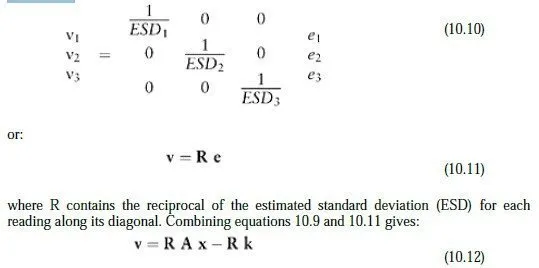
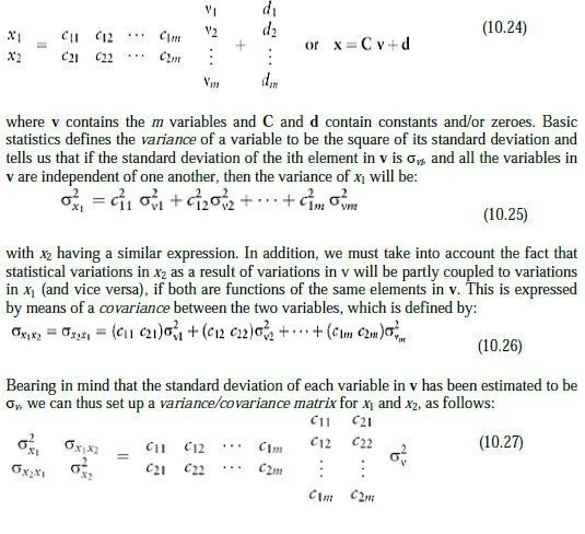
even if errors are present. Under these circumstances, we would expect the expression for to yield an indeterminate result. If the standard deviations in the initial readings were estimated correctly, then the RHS of equation 10.23 (commonly known as the estimated standard deviation scale factor) will evaluate to around unity, once the least-squares iteration has converged. If the factor is greater than unity, it indicates that the estimates appear to have been on the optimistic (i.e. small) side, given the remaining values; if less than unity then of course they were generally on the pessimistic (i.e. large) side. Note, however, that this is only an overall measure of the estimates; even if the value is unity, it is possible that some ESDs were too large and some too small. For each individual reading, though, the quoted ESD is known as the a priori estimate of its standard deviation and its ESD multiplied by σv is known as the a posteriori estimate of its SD. Assuming that the relative sizes of the ESDs are more or less correct, the best estimate for the actual standard deviation of the population in v is now given by σv, and the calculation can proceed to the next stage. If two variables, x1 and x2, can both be expressed as linear functions of m further variables, we can write this in the form:

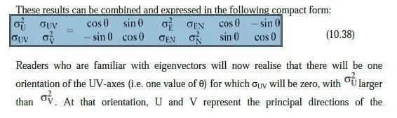
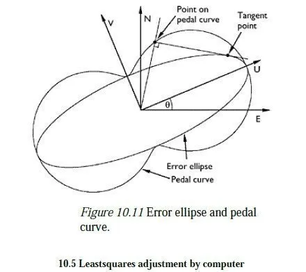
variance/covariance matrix for the point, with the maximum possible variance occurring in the U direction and the minimum in the V direction. The sizes of these principal variances are of course the two eigenvalues of the (symmetric) σEN matrix, with the U and V directions being given by the corresponding (orthogonal) eigenvectors. Alternatively, the sizes and directions of the principal variances can be obtained from a Mohrs circle construction, similar to that used in 2D stress calculations with variances in place of plane stress and covariances in place of shear stress. One standard deviation in any particular direction is of course given by the root of the variance in that direction, and normally, an engineer would simply be concerned to ensure that the largest standard deviation (i.e. the root of the largest eigenvalue of σEN) was adequately small for the job in hand. If needed, though, the standard deviations in other directions can be found, either by using equation 10.37 or via a Mohrs circle or more visually by means of the graphical construction shown in Figure 10.11. Here, an ellipse has been drawn on the UV-axes, with semi-major and semi-minor axes of σU and σV, respectively. This is the so-called error ellipse for the point. The size of one standard deviation in any direction is found by proceeding along a line in that direction until a perpendicular can be dropped which is tangential to the error ellipse. The resulting locus of points is known as the pedal curve of the error ellipse. As can be seen, the largest standard deviation is given by the major semi-axis of the error ellipse though there are also several other directions in which the standard deviation is very nearly as large.