10.1 Introduction
The term adjustment suggests that some form of cheating might take place during the process of converting surveying observations into results. This is not necessarily the case. As explained in Chapter 2, surveying observations always have two particular properties: 1 they contain errors (random, systematic and the occasional gross error); 2 the system of observations should always be such that more observations have been taken than would be strictly necessary to obtain the required result. This combination of properties means that no set of surveying observations is ever exactly consistent. If, for instance, the purpose of the observations is to fix the position of a new station, there will be no position which will exactly concur with all the data. All we can do is choose a position for the point which gives the best agreement with the observational data, and say that this is the most likely position of the point. The process of finding this best position is called adjustment. It only involves cheating if, in choosing a best position for the point, we ignore some of our observations simply because they do not appear to agree well with the other observations. The adjustment of large quantities of observations with several stations whose positions are unknown is a tedious job and is best done by computer. Several programs exist for this purpose and are able to take detailed account of what constitutes the best fit of the available data. The process they use is called least-squares adjustment and will be described later in this chapter. Often, though, it is adequate to use a simpler method which does not need elaborate computer software; one such method is called a Bowditch adjustment, and a simplified version of this adjustment is described below.
10.2 The Bowditch adjustment
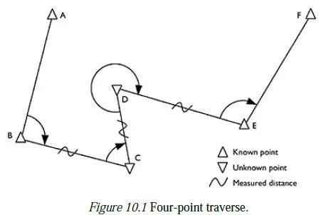
This adjustment method is best suited to a traverse (either in a horizontal plane or in the vertical direction). A basic version of the general method will be described with reference to a simple example. All distances will be assumed to be small, so that the (t−T) corrections described in the previous chapter can be ignored. A classic traverse to find the grid1 positions of two new stations is shown in Figure 10.1. The grid positions of stations A, B, E and F are already known, and the positions of stations C and D need to be found.
A scheme of observations to find these positions with some degree of redundancy is also shown in the figure. Angles are measured as shown, at stations B, C, D and E, and the horizontal distances BC, CD and DE are also measured. Note that the angles are measured using the previous station as the reference object; at D, for instance, C is used as the reference object, giving an observed angle CDE greater than 180°. Given these data, it is first possible to calculate the grid bearing of the line BA by simple trigonometry; then, by simply adding the measured angle ABC, the grid bearing of the line BC. Knowing this bearing and the length of the line BC,2 we can calculate a preliminary grid position for C. We can now repeat this process, to calculate preliminary grid positions for D and then for E. If all our readings were totally error-free, the preliminary grid position we would calculate for E would be exactly the same as its known grid position, which we already have as part of our data.
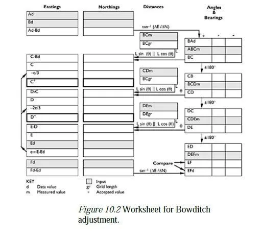
Inevitably, though, this will not be the case, and the fact that E has not turned out to be exactly where it is known to be means that the calculated positions for C and D are probably not correct either. In its simplest form, the Bowditch adjustment assumes that the errors in observation, which have given rise to the misplacement of E, are uniformly distributed throughout the traverse; so that C (which is 1/3 of the way through the traverse) should be adjusted by 1/3 of the amount which E must be adjusted, and D (which is 2/3 of the way through the traverse) should be adjusted by 2/3 of the same amount. Suppose, for instance, that the calculated position for E turns out to be 18 mm north and 12 mm west of the correct position; the best guess for the actual position of C is to subtract 6 mm from the northing and add 4 mm to the easting of the preliminary position. Likewise for D, we subtract 12 mm from the northing and add 8 mm to the easting. More elaborate forms of the adjustment also exist. Suppose, for instance, that the distance BC is 1/5 of the total distance BC+CD+DE. A better adjustment might be to adjust C by 1/5 of the adjustment needed for E, rather than by 1/3 as described above. In general, however, the extra work involved in these more elaborate adjustments does not result in a noticeably better set of co-ordinates for the unknown points. A calculation sheet for the application of a simple Bowditch adjustment to a two-point traverse of the type described above is shown in Figure 10.2. The calculation starts by filling in all the shaded squares, which are either data or observations. The next stage is to calculate all the bearings down the right-hand side of the sheet. The bearing of the line from B to A is calculated first, from the given grid co-ordinates. Adding the angle ABC3 to this value, and subtracting 360° if necessary, gives the bearing from B to C. Adding or subtracting 180° now gives the bearing from C to B, and the process can be repeated until a computed value of the bearing from E to F is obtained. This is then compared with the value which is computed from the known co-ordinates of E and F. If the agreement between these bearings is reasonable (not more than about twice the error that might be expected from a single angle measurement), the main calculation can now proceed. The next step is to convert all the observed horizontal distances to grid distances, filling in the spaces provided. This typically involves two operations:
1 Multiplying the horizontal distance calculated by an EDM device by the factor RE/(RE+h), where RE is the radius of the earth (6.381×10⁶ m) and h the height of the instrument above the ellipsoid (see Chapter 11, up to equation 11.6). Note that the ellipsoidal height of the instrument includes the height of the instrument above the geoid (i.e. its benchmark height), plus the height of the geoid above the ellipsoid in the area where the observation is made. Note also that this adjustment produces a negligible effect if h is less than about ±20 m.
2 Multiplying the distance calculated above by the local scale factor, as described in Section 9.3. For all but the largest traverses, this factor will be the same for all the distances in the traverse. Having done this, the easting and northing components of the vector BC can be calculated, using the computed bearing and distance from B to C. Adding the grid coordinates of B to this vector gives the preliminary co-ordinates for C. This process is then repeated to find preliminary co-ordinates for D and E as well. Finally, the co-ordinates which have just been computed for E are compared with its known co-ordinates, and the error or mis-closure is found. As described above, 1/3 of this mis-closure is now subtracted from C, and 2/3 from D, to yield accepted values (i.e. best guesses) for the co-ordinates of these two points.
A sample calculation of a Bowditch adjustment is given in Appendix E.
10.3 Leastsquares adjustment
The goal of adjustment is to choose the most likely co-ordinates for points whose positions are unknown, given the available readings. Once these co-ordinates have been chosen, the calculated angles and distances between these points and the fixed points will not all be exactly the same as those which were observed; any difference between each calculated and observed value must be presumed to be the error in the reading. Assuming that these errors have a statistically normal distribution, it can be shown that the most likely co-ordinates for the unknown points are those which yield the smallest value when the squares of all the errors are added together. The process of finding these co-ordinates is therefore known as least-squares adjustment. The exact process involved in least-squares adjustment4 is best explained by reference to a simple example. Suppose we wish to find the most likely easting and northing co-B, to take three measurements: (1) the distance AC, (2) the distance BC and (3) the angle BAC. Because of errors in these measurements, it will not in general5 be possible to find any position for C which will exactly concur with all the data. The process starts by taking a guessed position for C, and then seeing how this guess should be altered, in the hope of bringing the sum of the squares of the errors to a minimum. Taking Cs guessed co-ordinates to be (CN,CE), we can calculate the distance and bearing from A to this position for C (Figure 10.4):
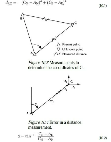
5 It is always possible that the errors in a set of observations will cancel each other out, to give the impression that they do not exist at all. Adding further redundancy to a set of observations reduces the likelihood of this undesirable possibility.
This calculated distance will in general not be equal to the measured distance, labelled as m1 in Figure 10.4. We define the difference between the calculated value and the measured value6 to be the current error for this reading, i.e.:
![]()
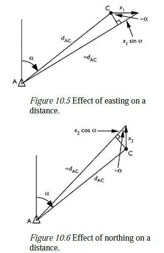
Now consider the two degrees of freedom we have for altering the position of C, denoted as x1 and x2 in Figure 10.4. In Figure 10.5, we can see that adding the quantity x1 to Cs easting will increase the calculated distance AC by approximately x1 sin α, provided x1 is small compared to dAC. Likewise in Figure 10.6, we can see that adding the quantity x2 to Cs northing will increase AC by approximately x2 cos α, again provided x2 is small.
6 The actual distance measured must first be reduced to the ellipsoid (see Chapter 11) and must then be multiplied by the local grid scale factor before being used in this equation.
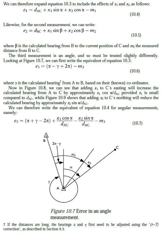
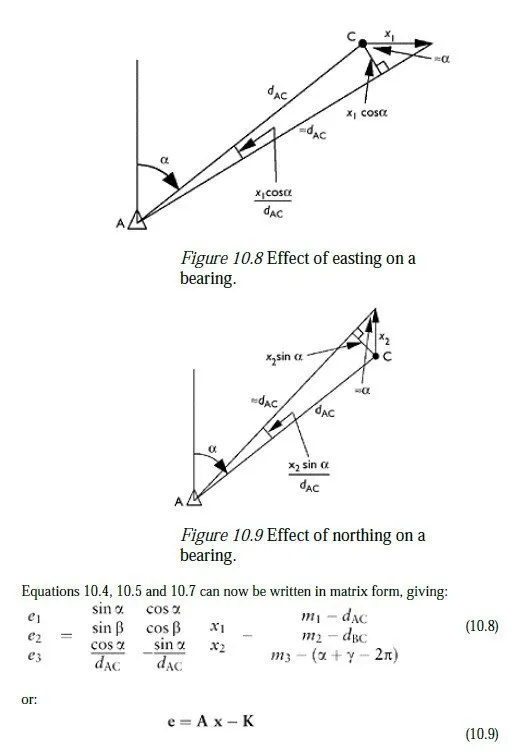
which shows how the 3D vector e is a linear function of the 2D vector x (provided the elements in x are small), with A and k containing only constants. Clearly the goal is to set the elements in x so as to make the components in e as small as possible.
However, there is one further complication to be overcome first; whereas e1 and e2 are distances, e3 is an angle, so its value cannot be compared directly with the other two values. Even in the case of the two distance measurements, it may be that one measurement is known to be much more accurate than the other, so that, say, a 1 mm error in measurement 1 is as likely as a 10 mm error in measurement 2. To overcome this problem, weighted errors are used in place of the actual errors, obtained by dividing each error by the estimated standard deviation which might be expected in repeated observations of the same measurement. We define a weighted vector v such that: