It is the usual practice of some designers to ignore the inertia forces of the mass of the gravity retaining wall in seismic design. Richards and Elms (1979) have shown that this approach is unconservative since it is the weight of the wall which provides most of the resistance to lateral movement. Taking into account all the seismic forces acting on the wall and at the base they have developed an expression for the weight of the wall Ww under the equilibrium condition as (for failing by sliding)
Eq. (11.89) is considerably affected by 8. If the wall inertia factor is neglected, a designer will have to go to an exorbitant expense to design gravity walls.
It is clear that tolerable displacement of gravity walls has to be considered in the design. The weight of the retaining wall is therefore required to be determined to limit the displacement to the tolerable limit. The procedure is as follows
1. Set the tolerable displacement Ad
2. Determine the design value of kh by making use of the following equation (Richards et al., 1979)
Passive Pressure During Earthquakes
Eq. (11.79) gives an expression for computing seismic active thrust which is based on the well known Mononobe-Okabe analysis for a plane surface of failure. The corresponding expression for passive resistance is
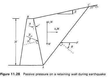
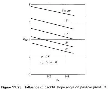
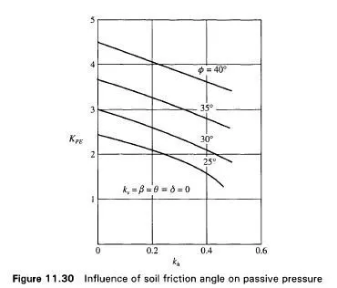
Fig. 11.28 gives the various forces acting on the wall under seismic conditions. All the other notations in Fig. 11.28 are the same as those in Fig. 11.25. The effect of increasing the slope angle P is to increase the passive resistance (Fig. 11.29). The influence of the friction angle of the soil (0) on the passive resistance is illustrated the Fig. 11.30.
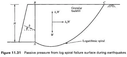
It has been explained in earlier sections of this chapter that the passive earth pressures calculated on the basis of a plane surface of failure give unsafe results if the magnitude of 6 exceeds 0/2. The error occurs because the actual failure plane is curved, with the degree of curvature increasing with an increase in the wall friction angle. The dynamic Mononobe-Okabe solution assumes a linear failure surface, as does the static Coulomb formulation.
In order to set right this anomaly Morrison and Ebelling (1995) assumed the failure surface as an arc of a logarithmic spiral (Fig. 11.31) and calculated the magnitude of the passive pressure under seismic conditions.
It is assumed here that the pressure surface is vertical (Q=0) and the backfill surface horizontal (B= 0). The following charts have been presented by Morrison and Ebelling on the basis of their analysis.
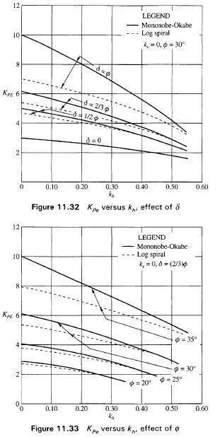
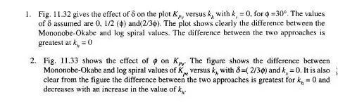
1 . Fig. 1 1 .32 gives the effect of 5 on the plot Kpe versus kh with kv = 0, for 0 =30°. The values of § assumed are 0, 1/2 (())) and(2/3<j)). The plot shows clearly the difference between the Mononobe-Okabe and log spiral values. The difference between the two approaches is greatest at kh = 0
2. Fig. 11.33 shows the effect of 0 on Kpg. The figure shows the difference between Mononobe-Okabe and log spiral values of K versus kh with 8=( 2/30) and kv = 0. It is also clear from the figure the difference between the two approaches is greatest for kh – 0 and decreases with an increase in the value of kh.